More with the Definite Integral¶

\[\int_a^b f(x) dx = \lim_{n \to \infty}\sum_{i = 1}^n f(x_i^*) \Delta x\]

WARM UP

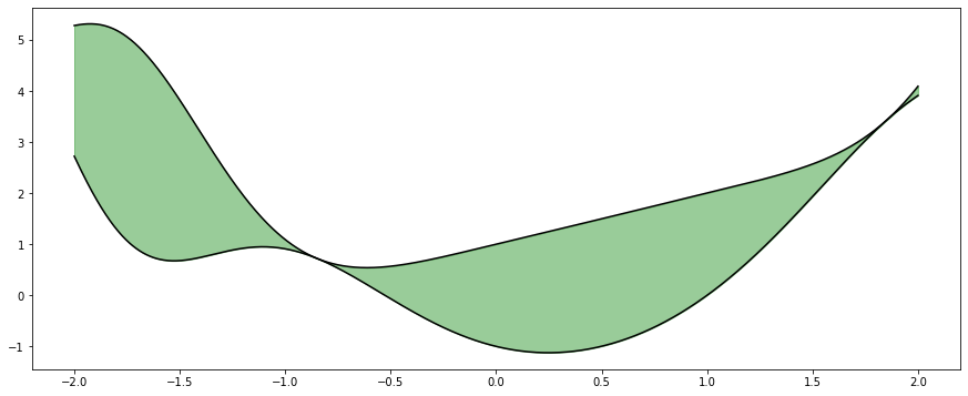
Evaluate the following definite integral. Interpret the integral as an area, and describe the region with a graph.

\[\int_{0} ^4 8x^3 - x^2 dx\]

Suppose the function $8x^3 - x^2$ represents the velocity of a car in miles per hour at a time $x$. Interpret the integral: $\int_{0} ^4 8x^3 - x^2 dx$
Suppose the function $8x^3 - x^2$ represents the rate at which water flows through a canal in ft$^3$. Interpret the integral: $\int_{0} ^4 8x^3 - x^2 dx$.

[1]:

%matplotlib inline
import matplotlib.pyplot as plt
import numpy as np
import pandas as pd

More Rules of Integrals¶

<td>$\displaystyle \int \ln(x)dx = x\ln(x) - x + C$</td>

<td>$\displaystyle \int \sin(x) dx = -\cos(x) + C$</td>
<td>$\displaystyle \int \cos(x) dx = \sin(x) + C$</td>
<td>$\displaystyle \int a^x dx = \frac{a^x}{\ln a} + C$</td>
</tr>

Your goal is to identify the appropriate rule to use for evaluating the given integral and then try to evaluate given definite integral. Plot the results and interpret the answer as an area under the curve.

$\displaystyle \int_0^{3\pi} \sin(x) dx$
$\displaystyle \int_0^4 \cos(x) + x^2 dx$
$\displaystyle \int_1^{10} \ln(x) - 2^x + 4$

[ ]:

[ ]:

[ ]:

[ ]:

Computing Solutions¶

We can use our computer to evaluate definite integrals. Consider the definite integral:

\[\int_0^4 x^2 dx\]

[2]:

import scipy.integrate as integrate

[3]:

x = np.linspace(0, 4, 1000)
def f(x): return x**2

[4]:

integrate.quad(f, 0, 4)

[4]:

(21.333333333333336, 2.368475785867001e-13)

[5]:

def f(x): return np.sin(x)

[6]:

integrate.quad(f, 0, 2*np.pi)

[6]:

(2.221501482512777e-16, 4.3998892617845996e-14)

Pure Symbolic Computing¶

This is the other side of the coin from using something like a Riemann sum, and we are dealing with symbols as opposed to numbers here. Accordingly, we introduce the symbolic representations using the library SymPy that is used for symbolic computing in Python.

[7]:

import sympy as sy

[8]:

#define the symbol
x = sy.Symbol('x')

[9]:

#define the function
def f(x): return x**2

[10]:

#evaluate the integral
#format is (function, (with respect to, start, stop))
sy.integrate(f(x), (x, 0, 4))

[10]:

$\displaystyle \frac{64}{3}$

\[\int_2^5 x^3 - \cos(x) + \ln(x) - e^{4x}\]

[11]:

##similar to with numbers(NumPy)
def f(x): return x**3 - sy.cos(x) + sy.log(x) + sy.exp(4*x)

[12]:

sy.integrate(f(x), (x, 2, 5))

[12]:

$\displaystyle - \frac{e^{8}}{4} - 2 \log{\left(2 \right)} + \sin{\left(2 \right)} - \sin{\left(5 \right)} + 5 \log{\left(5 \right)} + \frac{597}{4} + \frac{e^{20}}{4}$

Application I: Area Between Curves¶

Consider the functions $f(x) = x^2$ and $g(x) = \sqrt{x}$. How might we compute the area between the curves?

<img src = 'images/p8e1.png' />
</center>

A Creative Exercise¶

Definite Integral Art: Determining a beautiful region and its area.

[13]:

from ipywidgets import interact
import ipywidgets as widgets
def fun_plotter(a, b, c, d, e):
    def f(x): return a*x**2 + b*np.sin(c*x - d*x**2) + e
    def g(x): return a*x**2 - b*np.sin(c*x - d*x**2) - e
    x = np.linspace(-2, 2, 1000)
    plt.figure(figsize = (15, 6))
    plt.plot(x, f(x), color = 'black')
    plt.plot(x, g(x), color = 'black')
    plt.fill_between(x, f(x), g(x), where = (f(x) > g(x)), color = 'green', alpha = 0.4)

[14]:

interact(fun_plotter,
        a = widgets.IntSlider(1, min = -3, max = 3),
        b = widgets.IntSlider(1, min = -3, max = 3),
        c = widgets.IntSlider(1, min = -3, max = 3),
        d = widgets.IntSlider(1, min = -3, max = 3),
        e = widgets.IntSlider(1, min = -3, max = 3));

../_images/notebooks_08_more_with_integrals_26_0.png

Functions in Higher Dimensions¶

[15]:

from mpl_toolkits.mplot3d import Axes3D

[16]:

fig = plt.figure()
ax = fig.add_subplot(111, projection = '3d')
ax.set_xlabel('X', fontsize = 17, color = 'red')
ax.set_ylabel('Y', fontsize = 17, color = 'red')
ax.set_zlabel('Z', fontsize = 17, color = 'red')
plt.tight_layout()

../_images/notebooks_08_more_with_integrals_29_0.png

[17]:

x = np.linspace(-3,3,100)
y = np.linspace(-3,3,100)
def f(x,y): return -(x**2 + y**2)

[18]:

f(2, 4)

[18]:

-20

[19]:

fig = plt.figure()
ax = fig.add_subplot(111, projection = '3d')
ax.plot(x, y, f(x, y))
plt.tight_layout()

../_images/notebooks_08_more_with_integrals_32_0.png

[20]:

X, Y = np.meshgrid(x, y)
Z = f(X, Y)
fig = plt.figure()
ax = fig.add_subplot(111, projection = '3d')
ax.plot_surface(X, Y, Z)
plt.tight_layout()

../_images/notebooks_08_more_with_integrals_33_0.png

[21]:

X, Y = np.meshgrid(x, y)
Z = f(X, Y)
fig = plt.figure()
ax = fig.add_subplot(111, projection = '3d')
ax.contourf(X, Y, Z, zdir = 'x')
plt.tight_layout()

../_images/notebooks_08_more_with_integrals_34_0.png

[22]:

X, Y = np.meshgrid(x, y)
Z = f(X, Y)
fig = plt.figure()
ax = fig.add_subplot(111, projection = '3d')
ax.plot_wireframe(X, Y, Z)
ax.contour(X, Y, Z, zdir = 'x', offset = -3)
ax.contour(X, Y, Z, zdir = 'y', offset = 3)
ax.contour(X, Y, Z, zdir = 'z', offset = -18)
plt.tight_layout()

../_images/notebooks_08_more_with_integrals_35_0.png

[24]:

import seaborn as sns
grid = np.linspace(-3, 3, 10)
X, Y = np.meshgrid(grid, grid)
a = np.random.randint(1, 6, 64).reshape(8,8)
plt.figure(figsize = (6,6))
sns.heatmap(a, annot = True,
            linewidths = 0.5, cmap="BuGn",
            cbar = False,
            square = True)
b, t = plt.ylim() # discover the values for bottom and top
b += 0.5 # Add 0.5 to the bottom
t -= 0.5 # Subtract 0.5 from the top
plt.ylim(b, t)
plt.tight_layout()
plt.title('Heights of Rectangles on a Grid')

[24]:

Text(0.5, 1, 'Heights of Rectangles on a Grid')

../_images/notebooks_08_more_with_integrals_36_1.png

[25]:

l = min(top)

-----------------------------------------------------------
NameError                 Traceback (most recent call last)
<ipython-input-25-a4ac4e2489a4> in <module>
----> 1 l = min(top)

NameError: name 'top' is not defined

[ ]:

m = max(top)

[30]:

x = np.arange(8)
y = np.arange(8)
X, Y = np.meshgrid(x, y)
x, y = X.ravel(), Y.ravel()

top = 2*x**2 - x*y
bottom = np.zeros_like(top)
width = depth = 1


# cmap = cm.get_cmap('jet')
l = min(top)
m = max(top)

fig = plt.figure(figsize = (20, 15))
ax = fig.add_subplot(121, projection = '3d')
ax.bar3d(x, y, bottom, width, depth, top, alpha = 0.5, color = [cmap((k - l)/m) for k in top])
plt.tight_layout()
ax = fig.add_subplot(122, projection = '3d')
ax.bar3d(x, y, bottom, width, depth, top, alpha = 0.5, color = [cmap((k - l)/m) for k in top])
ax.view_init(elev = 10., azim = 180)

# plt.tight_layout()

-----------------------------------------------------------
NameError                 Traceback (most recent call last)
<ipython-input-30-0ebf899eab51> in <module>
     15 fig = plt.figure(figsize = (20, 15))
     16 ax = fig.add_subplot(121, projection = '3d')
---> 17 ax.bar3d(x, y, bottom, width, depth, top, alpha = 0.5, color = [cmap((k - l)/m) for k in top])
     18 plt.tight_layout()
     19 ax = fig.add_subplot(122, projection = '3d')

<ipython-input-30-0ebf899eab51> in <listcomp>(.0)
     15 fig = plt.figure(figsize = (20, 15))
     16 ax = fig.add_subplot(121, projection = '3d')
---> 17 ax.bar3d(x, y, bottom, width, depth, top, alpha = 0.5, color = [cmap((k - l)/m) for k in top])
     18 plt.tight_layout()
     19 ax = fig.add_subplot(122, projection = '3d')

NameError: name 'cmap' is not defined

../_images/notebooks_08_more_with_integrals_39_1.png

[31]:

import ipywidgets as widgets
from ipywidgets import interact
def bar_approximator(elev, azim):
    fig = plt.figure(figsize = (20, 15))
    ax = fig.add_subplot(111, projection = '3d')
    ax.bar3d(x, y, bottom, width, depth, top, alpha = 0.5, color = [cmap((k - l)/m) for k in top])
    ax.view_init(elev = elev, azim = azim)

[32]:

interact(bar_approximator,
        elev = widgets.IntSlider(0, min = 0, max = 360),
        azim = widgets.IntSlider(0, min = 0, max = 360))

-----------------------------------------------------------
NameError                 Traceback (most recent call last)
~/opt/anaconda3/lib/python3.7/site-packages/ipywidgets/widgets/interaction.py in update(self, *args)
    254                     value = widget.get_interact_value()
    255                     self.kwargs[widget._kwarg] = value
--> 256                 self.result = self.f(**self.kwargs)
    257                 show_inline_matplotlib_plots()
    258                 if self.auto_display and self.result is not None:

<ipython-input-31-f36301c2491b> in bar_approximator(elev, azim)
      4     fig = plt.figure(figsize = (20, 15))
      5     ax = fig.add_subplot(111, projection = '3d')
----> 6     ax.bar3d(x, y, bottom, width, depth, top, alpha = 0.5, color = [cmap((k - l)/m) for k in top])
      7     ax.view_init(elev = elev, azim = azim)

<ipython-input-31-f36301c2491b> in <listcomp>(.0)
      4     fig = plt.figure(figsize = (20, 15))
      5     ax = fig.add_subplot(111, projection = '3d')
----> 6     ax.bar3d(x, y, bottom, width, depth, top, alpha = 0.5, color = [cmap((k - l)/m) for k in top])
      7     ax.view_init(elev = elev, azim = azim)

NameError: name 'cmap' is not defined

[32]:

<function __main__.bar_approximator(elev, azim)>

../_images/notebooks_08_more_with_integrals_41_2.png

[28]:

# x = np.linspace(0, 1, 100)
# def f(x): return x**2
# def g(x): return np.sqrt(x)

# fig, ax = plt.subplots(nrows = 1, ncols = 3, figsize = (16, 6))
# ax[0].plot(x, f(x), color = 'black')
# ax[0].fill_between(x, f(x), color = 'orange', alpha = 0.6)
# ax[0].set_title('$f(x) = x^2$')

# ax[1].plot(x, g(x), color = 'black')
# ax[1].fill_between(x, g(x), color = 'green', alpha = 0.5)
# ax[1].set_title('$g(x) = \sqrt{x}$')

# ax[2].plot(x, g(x), color = 'black', label = '$g(x)$')
# ax[2].plot(x, f(x), linestyle = '--', color = 'black', label = '$f(x)$')
# ax[2].fill_between(x, f(x), g(x), color = 'yellow', alpha = 0.6)
# ax[2].fill_between(x, f(x), color = 'lightblue', alpha = 0.5)
# ax[2].legend()
# plt.savefig('images/p8e1.png')

[1]:

import name_caller as namer

[3]:

namer.your_turn()

[3]:

'What do you think Seba'

[ ]:

$\displaystyle \int x^n dx = \frac{x^{n+1}}{n+1} + C$

$\displaystyle \int e^{ax} dx = \frac{1}{a} e^{ax} + C$